PITLAKQ Tutorial#
Preliminaries#
This tutorial assumes that you have installed PITLAKQ properly and can run it from the command line as explained in the section A Python Program.
Running Python Scripts#
Some of the task are done via Python scripts. There are two options:
Run the script saved in a file from the command-line via
python my_script.pyRun from inside a Jupyter notebook.
For the second option type:
jupyter lab
A browser window will open.
Click on the drop-down menu New and select Python 3.
This will open a new notebook.
Enter the Python commands into a cell and type <Shift><Enter>.
Create a new project#
The first thing we need to do is to create new, still empty, project.
Create a new project named my_project by typing:
pitlakq create my_project
Now you should have a directory inside your models directory with a layout
that looks like this:
pitlakq_tut
|
+---balance
+---input
|   +---main
|   +---w2
+---output
|   +---sediment
|   +---w2
+---postprocessing
+---preprocessing
    +---input
    +---output
    +---tmp
Preprocess the bathymetry data#
The bathymetry of the lake needs to be discretized. CE-QUAL-W2 and therefore PITLAKQ is two-dimensional along x and z. The y-direction is parametrized as cell width. Let’s assume we have a lake that looks like the following picture.
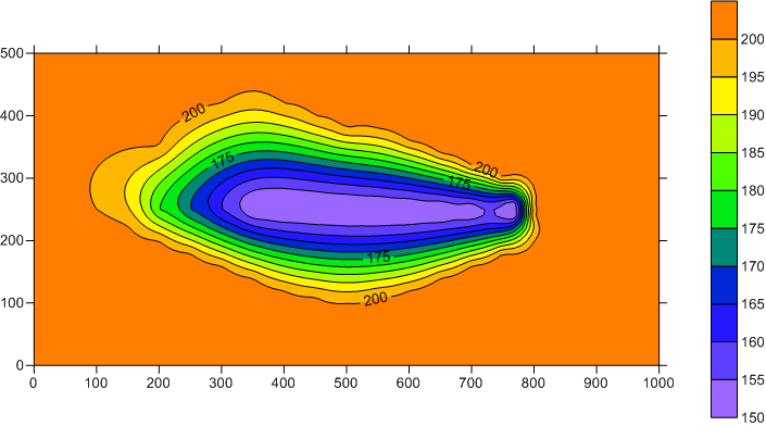
We save the gridded data that where used to generate this contour plot in a
a SURFER 6 text file named bath_asci.grd
(this default name can be changed with configuration options if needed).
The file content look like this:
DSAA
100 51
0 1000
0 500
150.03254732465 214.3417454463
202.0000000052914 202.5142874143128 203.0243218381507
Currently, PITLAKQ only supports this file format. Adding more formats is possible.
If there are many points with lake bottom elevation data, linear interpolation may be accurate enough. PITLAKQ provides a pre-processing tool for creating a SURFER 6 text file with linear interpolation.
These are the data points that were used to create the above contour map:
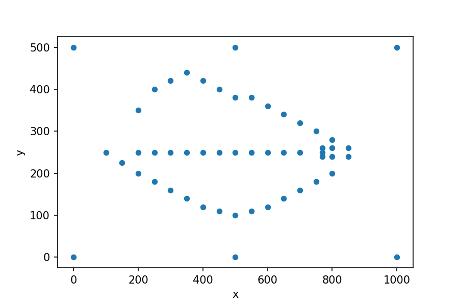
You can create this plot with this code:
from pitlakq.preprocessing.create_bathgrid import show_points

show_points(project_name='pitlakq_tut', bath_data_file_name='bath_data.txt')
The file named bath_data.txt with the data looks like this:
x y z
100 250 200
150 225 200
200 200 200
250 180 200
300 160 200
350 140 200
400 120 200
450 110 200
500 100 200
This Python program creates the SURFER file for the project pitlakq_tut,
using 100 grid locations in x and 51 grid locations in y direction:
from pitlakq.preprocessing import create_bathgrid

create_bathgrid.main('pitlakq_tut', 'bath_data.txt', num_x=100, num_y=51)
The resulting grid file allows to generate this contour plot:
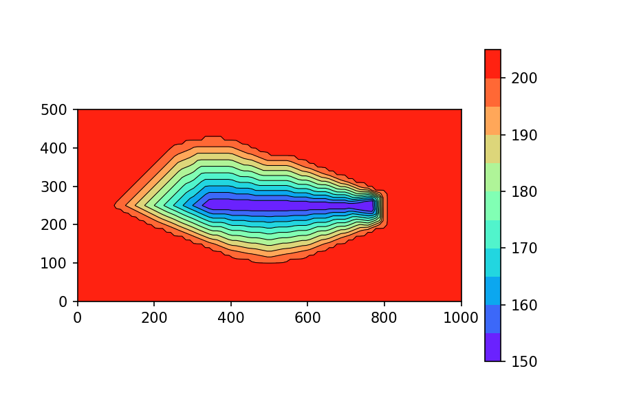
You can create this plot with this code:
from pitlakq.preprocessing.create_bathgrid import show_contours

show_contours(project_name='pitlakq_tut',
              bath_data_file_name='bath_data.txt',
              num_x=100, num_y=51, show_plot=True)
This looks similar to the SURFER-generated contour plot. An analyses shows that the surface area differs by about 6% and the lake volume by about 9%. The differences will be smaller for denser data points.
This tool can also be used to apply a different griding algorithm or program:
Save the griding result in x-y-z format such as in the file
bath_data.txtwith high resolution, i.e. many data points.Apply the tool as described above with many interpolation points in x and y direction.
Alternatively, you can save the griding results directly in the SURFAER text format.
Now, we specify how our lake grid is going to look like.
PITLAKQ currently supports either East-West or North-South directed grid
layouts.
This due to the (here not covered coupling to regularly gridded groundwater
models.
We place a file called reservoir.txt inside our directory
preprocessing/input.
This is the file content:
Columns	RW
1	100
2	200
3	300
4	400
5	500
6	600
7	700
8	800
9	900
Layers ZU
1 150
2 151
3 152
4 153
5 154
6 155
7 156
8 157
9 158
10 159
11 160
12 161
13 162
14 163
15 164
16 165
17 166
18 167
19 168
20 169
21 170
22 171
23 172
24 173
25 174
26 175
27 176
28 177
29 178
30 179
31 180
32 181
33 182
34 183
35 184
36 185
37 186
38 187
39 188
40 189
41 190
42 191
43 192
44 193
45 194
46 195
47 196
48 197
49 198
50 199
51 200
We have 9 columns running from East to West with a distance of 100 each. We could vary the distance for each column (or segment). We also choose a equi-distant discretization in the vertical with 1 m per layer for 50 layers.
We supply more information in the file preprocessing.yaml:
bathymetry:
    initial_water_surface:
        value: 185
    max_water_surface:
        value: 200
    orientations:
        value: [1.57]
This file is in the YAML format. The entry orientations here says that our
first (sub)lake (we only have one sub-lake, which takes up the total lake) is in
East-West direction.
Now we start our preprocessing program in a similar fashion as setting up a new
project. Create file called do_preprocessing.py with this content:
from pitlakq.preprocessing import preprocess

preprocess.main('pitlakq_tut')
Replace the name pitlakq_tut with your project name. e.g.
my_project.
Run it: python do_preprocessing.py. If everything goes well you
will have a file named bath.nc in the output directory under
preprocessing. This file bath.nc will be used as input for our model
run. It is in netCDF format.
The file bath.nc can be converted into a human readable format with
ncdump bath.nc:
netcdf bath {
dimensions:
        segment_lenght = 10 ;
        layer_height = 52 ;
variables:
        double segment_lenght(segment_lenght) ;
        double starting_water_level(segment_lenght) ;
        double segment_orientation(segment_lenght) ;
        double layer_height(layer_height) ;
        double cell_width(layer_height, segment_lenght) ;
data:

 segment_lenght = 100, 100, 100, 100, 100, 100, 100, 100, 100, 100 ;

 starting_water_level = 200, 200, 200, 200, 200, 200, 200, 200, 200, 200 ;

 segment_orientation = 9.99, 1.57, 1.57, 1.57, 1.57, 1.57, 1.57, 1.57, 1.57,
    9.99 ;

 layer_height = 1, 1, 1, 1, 1, 1, 1, 1, 1, 1, 1, 1, 1, 1, 1, 1, 1, 1, 1, 1,
    1, 1, 1, 1, 1, 1, 1, 1, 1, 1, 1, 1, 1, 1, 1, 1, 1, 1, 1, 1, 1, 1, 1, 1,
    1, 1, 1, 1, 1, 1, 1, 1 ;

 cell_width =
  0, 0, 0, 0, 0, 0, 0, 0, 0, 0,
  0, 75.6157364131951, 145.089953029845, 222.101772341138, 279.100893272702,
    279.22978559541, 222.26566587868, 141.54165990374, 27.8009873136653, 0,
  0, 64.9264248803291, 139.74267671092, 215.582246846721, 274.371310775368,
    274.382373960408, 216.115799371682, 134.929618517385, 23.2367196470327, 0,
...
We can visualize our lake grid. Create a file called do_show_bath.py with
this content:
from pitlakq.postprocessing import show_bath

show_bath.main("output/bath.nc", bottom=150)
Run it: python do_show_bath.py. You should see a picture like
this:
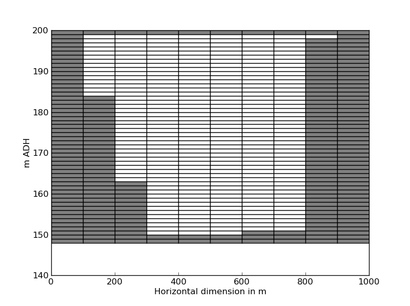
Lake Bathymetry#
Copy the file bath.nc into the directory /tut/pitlakq_tut/input/w2/.
Create the main input file#
Now we need to create input files. PITLAKQ has many hundreds of input
variables. Fortunately, for many applications sensible default will values can
be used. In the template directory (see your .pitlakq for its
location). You will find many templates of input files that contain default
values. The following input files contain only a minimal, site-specific data set.
Most of the input is taken from the defaults. Since we do only a very simple
model (hydrodynamics only, no inflow, no precipitation no evaporation) to show
the general principal how PITLAKQ works, this is approach is useful. For
real-world applications the amount of (different) input data is typically much
larger. We look at the many options that are involved when water quality
calculations that couple chemical and biological process or treatment, erosion or
sediment interactions come into play in later tutorials.
The input files are either in YAML or CSV (text in columns) format. Both
formats are easily readable by humans and computers. The YAML files use the
so called !File directive, which allows to include YAML into other YAML
by referencing them rather than copying their content. This means the same file
can be used from several other YAML files. Furthermore, the input can be spread
over as many or a as few input files as desired. This gives great flexibility how
to arrange the model best for each specific task.
This is a minimal PITLAKQ input file with information about the whole model.
For an overview of all available options see the file pitlakq.yaml in the
directory <install_dir>/pitlakq/templates
(See Initializing PITLAKQ for details about where this path is
located.):
general:
    start:
        value: 01.01.1998
    gw_start:
        value: 01.01.1998
    lake_time_step:
        value: .1
    number_of_gw_time_steps:
        value: 120
    dump_input:
        value: False
lake:
    max_water_surface:
        value: 200.0
    deepest_segment:
        value: 8
It is located in the directory where all your PITLAKQ projects are:
<my_project_name>/input/main/pitlakq.yaml. Change <my_project_name>
to the name of your project.
This file has two groups general and lake.
There are several more groups.
But since we can use the default values from <install_dir>\pitlakq\templates
we don’t need to repeat them here.
All values must be indented by four space, not tabs.
Best is to turn the option in your editor to display non-printing characters.
For example, with Notepad++ the menu View | Show Symbol | Show White Space and
TAB allows you to make them visible.
We always edit the attribute value there can be more attributes like
unit but we don’t use them here.
The value for start is 01.01.1998.
Note: Currently, dates always have to be in DD.MM.YYYY-format. Other formats
would be possible but are not implemented yet. There is a second date for the
start called gw_start. This is doe to historical reasons. Please use
gw_start plus number_of_gw_time_steps to specify actual model run.
A gw_time_step is by default one calendar month long. So 120 month
will be exactly 10 years. Leap years are considered. The option dump_input
make PITLAKQ to stop after reading all inputs to give you the possibility to
dump the input, which is combination of the defaults and the user settings
into one big YAML file. While this can take several seconds, it can be
interesting to see these data.
The group lake allows you to give more information about the lake model.
Here we only provide max_water_surface and deepest_segment. The later
could be induced from the bathymetry data in bath.nc but for various
reasons it can be supplied here.
Create a W2 input file#
The file <my_project_name>/input/w2/w2.yaml has more entries:
general:
    titel:
        value: A simple PITLAKQ test model
bounds:
    number_of_segments:
        value: 10
    number_of_layers:
        value: 52
    number_of_constituents_segments:
        value: 10
    number_of_constituents_layers:
        value: 52
times:
    start:
        value: 01.01.1998
    end:
        value: 31.01.2009
---
!File
    name: bath.nc
    format: netcdf
    group_name: bathymetry
---
bathymetry:
    starting_water_level:
        value: 195.0
---
branch_geometry:
    branch_name:
        value:
            - test lake                         # no w2 variable
    branch_upstream_segments:
        value:
            - 2
    branch_downstream_segments:
        value:
            - 8


waterbody_coordinates:
    latitude:
        value: -33.21 # degrees
    longitude:
        value: 116.093  # degrees
    bottom_elevation:
        value: 150.0

tributaries:
    number_of_tributaries:
        value: 1
    tributary_names:
        value:
            - mytribname
    tributary_segment:
        value:
            - 5

ice_cover:
    allow_ice_calculations:
        value: False

initial_conditions:
    initial_temperature:
        value: 10 # isothermal
    temperature:
        value: 10.0
    ice_thickness:
        value: 0.0

initial_concentrations:
    tracer:
        value: 10.0

---
!File
    name: meteorology.txt
    format: columns_whitespace
    group_name: meteorology


---
!File
    name: precipitation.txt
    format: columns_whitespace
    group_name: precipitation


---
!File
    name: precipitation_temperature.txt
    format: columns_whitespace
    group_name: precipitation_temperature


---
!File
    name: precipitation_concentration.txt
    format: columns_whitespace
    group_name: precipitation_concentration
Most of the information in this file are handed down to CE-QUAL-W2.
In fact, the file <install_dir>/pitlakq/templates/w2.yaml has an attribute
w2_code_name for most of the entries. This corresponds to variable name
in CE-QUAL-W2. Therefore, more information about each of this entries can be
found in the CE-QUAL-W2 manual or in FORTRAN source code.
We provide a model title and detailed information about the model bounds. Here
we just repeat the 10 by 52 setup from our bath.nc. These dimensions will be
used to check if other input values we will specify later are of the correct
shape.
Then we start a new stream with --- and include the file bath.nc with
help of the directive !File- This file is in netCDF format and we would
like it to be in the group bathymetry. The specification of this group
allows to override parts of the data in bath.nc. We do this by providing
an different value for the starting water label and set starting_water_level
in the group bathymetry to 195.0 (meters). No need to go into the netCDF
file and change data there.
The group branch_geometry provides information for each branch. We only
have one branch in this case. Multi-branch setups are possible but more
complicated and only recommend for complex cases such as complex geometries
or large difference in lake water levels. The branch_upstream_segments is
typically 2 for the first branch. The value for
branch_downstream_segments is 8 instead of 9, which would be the
last active segment. Looking at the lake cells (Lake Bathymetry),
we can see that the last segment in only one meter deep. This means setting
branch_upstream_segments to 9 works only if the water level is at
200 m. Below this segment is dry and CE-QUAL-W2 terminates with an error
message.
The waterbody_coordinates are in degrees of latitude and longitude, where
the southern hemisphere gets negative values for latitude. Even though, we don’t
have any tributary inflow yet, wen need (for input reasons in CE-QUAL-W2)
provide on tributary, which we do in group tributaries. As we will see,
we just put a value of zero for inflow to turn it off. We don’t want to
calculate the ice cover and therefore set allow_ice_calculations in the
group ice_cover to False.
We use very simple initial conditions. Setting initial_temperature to
positive value uses this value for isothermal conditions throughout the entire
lake. Using a -1 or -2, we can specify a one-dimensional or
two-dimensional temperature distribution in temperature. That is also the
reason we need to repeat this temperature. Similarly, even
though we turned ice calculations of, we need to set ice_thickness because
the default value has different dimensions. Similarly, we set the
initial_concentrations of a specie tracer to 10.00 even though, we
don’t calculate species yet.
Now we include more files using the directive !File. Let’s have a look at
these files.
The meteorology file provides input data for:
air temperature,
dew point temperature,
wind speed,
wind direction and
cloud cover
The time resolution can be as fine as desired up to one minute. Finer resolution would be possible but the input format does not support it yet.
date            time  air_temperature  dewpoint_temperature  wind_speed  wind_direction  cloud_cover
01.03.1997     00:00            14.4                 6.80       3.06           2.27           0
01.03.1997     01:00            13.9                 7.00       3.06           2.09           0
01.03.1997     02:00            13.4                 7.00       2.50           2.09           0
01.03.1997     03:00            12.8                 7.10       1.39           2.09           0
01.03.1997     04:00            12.8                 7.10       1.39           2.27           0
01.03.1997     05:00            13.1                 7.40       2.50           2.09           0
01.03.1997     06:00            13.0                 7.50       1.39           2.27           0
01.03.1997     07:00            13.9                 7.90       2.22           2.09           0
01.03.1997     08:00            15.3                 8.10       3.06           1.92           0
The precipitation file is simpler. It only has the entry for precipitation in m/s:
date            time  precipitation
01.03.1997     00:00      0.000e+00
01.03.1997     01:00      0.000e+00
01.03.1997     02:00      0.000e+00
01.03.1997     03:00      0.000e+00
01.03.1997     04:00      0.000e+00
01.03.1997     05:00      0.000e+00
01.03.1997     06:00      0.000e+00
01.03.1997     07:00      0.000e+00
01.03.1997     08:00      0.000e+00
Likewise, the precipitation temperature:
date        time       precipitation_temperature
01.01.2001  00:00         15.5
02.01.2001  00:00         15.5
01.02.2001  12:00:00.0    15.5
02.02.2001  12:00:00.0    15.5
31.12.2020  00:00:00.0    15.5
31.12.2100  00:00:00.0    15.5
and the concentration:
date        time      tracer
01.01.1993  00:00:00.0          0.0
01.01.2020  00:00:00.0          0.0
For each entry in tributary_names, we need to specify:
<mytribname>_inflow.txt
<mytribname>_temperature.txt
<mytribname>_concentration.txt
Replace <mytribname> with name(s) you used.
We don’t have any inflow:
date            time  tributary_inflow
01.01.1997     00:00      0.0
01.01.2011     00:00      0.0
Therefore, data in the temperate file:
date        time       tributary_temperature
01.01.1997  00:00         15.0
01.01.2011  00:00         15.0
and the concentration file:
date    time    tracer
01.03.1997      00:00:00.0      0.0
01.01.2020      00:00:00.0      0.0
are ignore.
The specification of not-used values can be a bit misleading. PITLAKQ follows CE-QUAL-W2 as close as possible to allow the of the CE-QUAL-W2’s manual as much as possible.
Looking at results#
Run your model with pitlakq run <project_name>. The calculation should be
finished after a few minutes. Now we can visualize the temperature at one point
over time. Create a file called do_show_temp.py with this content:
from pitlakq.postprocessing import depth_time_contour

species=[{"name": "t2", "levels": "auto"}]
depth_time_contour.main("../output/w2/out.nc", species=species, location=5)
This assumes the file is located in the postprocessing directory of your
project. Now run it:
python do_show_temp.py
You should see a picture like this:
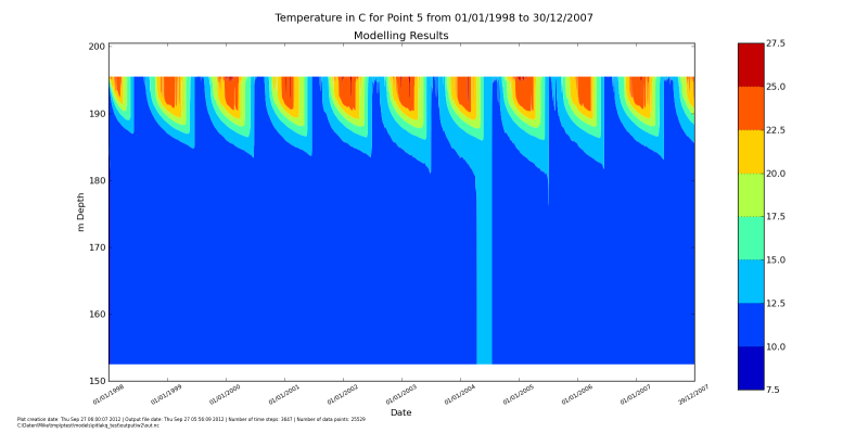
Turning on precipitation#
You can see that the water level does not change over the whole runtime of the
model. This is due to fact that there no sources or sinks to our lake. Let’s add
some precipitation. Add this to your w2.yaml file:
calculations:
    precipitation_included:
        value: True
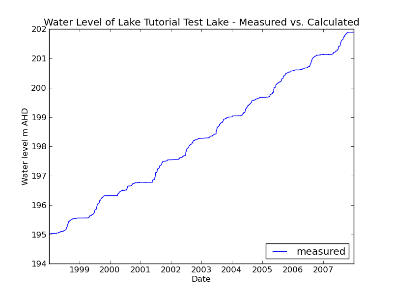
Now re-run your model and look at the water level that is printed to the screen. It should drop with each time step. We can visualize the lake water level with this script:
from pitlakq.postprocessing import waterlevel


waterlevel.main("../output/w2/out.nc", lake_name="Tutorial Test Lake",
                loc="lower right")
This assumes the file is located in the postprocessing directory of your
project. Now run it:
python do_show_wl.py
You should see a picture like this:
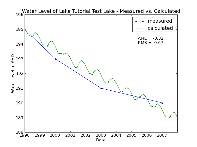
Adding evaporation#
Now we also turn on evaporation:
calculations:
    evaporation_included_in_water_budget:
        value: True
Now re-run your model and look at the water level that printed to the screen. It should drop with each time step. Now we also us measured water level data to compare to our calculations:
date            level
01.01.1998       195.0
01.01.2000       193.0
01.01.2003       191.0
01.01.2007       190.0
We modify our script a bit:
from pitlakq.postprocessing import waterlevel


waterlevel.main("../output/w2/out.nc", lake_name="Tutorial Test Lake",
                measured_values_path="measured_wl.txt")
and run it:
python do_show_wl_measured.py
You should see a picture like this:
Adding inflow#
mytribname_inflow.txt
We add some inflow:
date            time  tributary_inflow
01.01.1997     00:00      0.005
01.01.2011     00:00      0.0
Re-run the model and see how the water level in the lake changes.
Charge balancing#
The initial lake composition and all inflows need to be charge balanced. This is important because the pH value is calculated via the charge. PITLAKQ offers tools to make charge balancing of inflows easier, especially if many inflow time steps need to be charged.
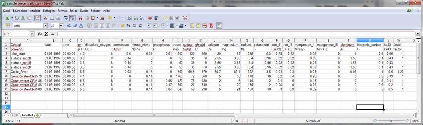
We supply measured concentrations for all inflows in an CSV
sample_concentration.csv file:
Cequal;date;time;ph;dissolved_oxygen;ammonium;nitrate_nitrite;phosphorus;tracer;sulfate;chlorid;calcium;magnesium;sodium;potassium;iron_II;iron_III;manganese_II;manganese_III;aluminium;inorganic_carbon;ks43;factor
phreeqc;;;pH;O(0);Amm;N(+5);P;skip;Sulfat;Cl;Ca;Mg;Na;K;Fe(+2);Fe(+3);Mn(+2);Mn(+3);Al;C;ks43;factor
lake_start;01.03.1997;00:00:00;4.2;8;0.5;0.34;0.01;1200;120;550;20;59;255;5.3;0.28;0.52;0.25;0;4;0.5;0.56;1
surface_runoff;01.03.1997;00:00:00;3.6;8;0.14;0;0;50;35;0;2.55;3.85;5.4;0.96;0.02;0.02;0.09;0;1.55;0.1;0.43;1
surface_runoff;01.05.1998;00:00:00;3.6;8;0.14;0;0;50;35;0;2.55;3.85;5.4;0.96;0.02;0.02;0.09;0;1.55;0.1;0.43;1
surface_runoff;01.07.1999;00:00:00;3.6;8;0.14;0;0;50;35;0;2.55;3.85;5.4;0.96;0.02;0.02;0.09;0;1.55;0.1;0.43;1
Collie_River;01.03.1997;00:00:00;6.7;8;0.03;0.18;0;1500;60.5;879;30.7;83.1;392;3.6;0.01;0.3;0.08;0;0.06;1;0.6;1.23
Groundwater-CRM-79;01.03.1997;00:00:00;4.1;8;0;0.11;0;1760;72;860;5;63;470;10;0.2;0.4;0.26;0;0;0.5;0.19;1
Groundwater-CRM-85;01.03.1997;00:00:00;5.6;8;0;0.11;0.05;420;75;130;2;3;110;2;0.1;0;0.18;0;0;5;0.11;1
Groundwater-CRM-86;01.03.1997;00:00:00;4.5;8;0;0.11;0.17;560;27;310;4;20;170;2;0.05;0;0.09;0;0;0.5;0.2;1
Groundwater-CRM-89;01.03.1997;00:00:00;5.6;8;0;0.11;0.04;640;59;290;5;21;180;18;3;0.9;0.32;0;0;5;0.5;1
Opened in a spreadsheet program, it looks like this:
Now we create a script to start our charge balancing run:
import datetime
import os

from pitlakq.preprocessing import charge_tributaries

# Get current working directory.
base = os.getcwd()
# Build absolute path.
in_file_name = os.path.join(base, 'sample_concentration.csv')
# Start charging.
charge_tributaries.main(project_name='pitlakq_tut',
                        in_file_name=in_file_name,
                        out_dir=base,
                        charging_species='Cl',
                        last_date=datetime.datetime(2012, 1, 5))
and execute it:
python do_trib_charge.py
This will generate the files:
Collie_River.txtGroundwater-CRM-79.txtGroundwater-CRM-85.txtGroundwater-CRM-86.txtGroundwater-CRM-89.txtlake_start.txtsample_concentration_.txtsurface_runoff.txt
that contain this kind of information:
      date       time                        ph          dissolved_oxygen                  ammonium           nitrate_nitrite ...
01.03.1997  00:00:00                   6.70000                   8.00000                   0.03000                   0.18000  ...
05.01.2012  00:00:00                   6.70000                   8.00000                   0.03000                   0.18000  ...
Tributaries that are in contact with atmosphere my exhibit some deviations in
terms of carbon concentration. If the acid capacity is known, it can be used
as additional information. We run the script do_check_trib_charge.py:
import os
from pitlakq.preprocessing import check_kb_balance

# Get current working directory.
base = os.getcwd()
# Build absolute path.
in_file_name = os.path.join(base, "Collie_River.txt")
# Specify project name.
project_name  = "pitlakq_tut"
target_ph = 4.3
# Start charging.
check_kb_balance.main(project_name,in_file_name, target_ph)
python do_check_trib_charge.py
It titrates the water toward a pH of 4.3 and compares the used amount acid with of the measured value for this titration. It will output something like this:
            date  calc  meas ratio
      01.03.1997  0.60  0.60  1.00
      05.01.2012  0.60  0.60  1.00
min 0.0018992835095
max 0.0018992835095
average 0.0018992835095
abs average 0.0018992835095
run time 0.0929999351501
If the ratio is different from 1.0 you may adjust the value for factor in
sample_concentration.csv for the Collie River water, re-run
do_trib_charge.py and do_check_trib_charge.py. Repeat until the
the ratio approaches 1.0. This excises has to be supported by fundamental
chemical understanding of the underlying process.
Water quality calculations#
To do water quality calculations, we need to add more entries to our
pitlakq.yaml:
general:
    start:
        value: 01.01.1998
    gw_start:
        value: 01.01.1998
    lake_time_step:
        value: .1
    number_of_gw_time_steps:
        value: 120
    dump_input:
        value: False
lake:
    lake_calculations:
        value: True
    max_water_surface:
        value: 200.0
    deepest_segment:
        value: 8
    kinetics:
        value: True

phreeqc:
    lake_active_const_names:
        value:
            - na
            - cl
            - dox
            - no3
            - nh4
            - po4
            - ca
            - so4
            - mg
            - mn
            - ka
            - al
            - tic
            - fe3
            - mn3
            - fe
    rates:
        value:
            - fe
            - fe3
            - mn
            - mn3
            - so4

    mineral_rates:
        value:
            - feoh3
    lake_active_minerals_names:
        value:
            - feoh3
            - aloh3
            - po4precip
    charge:
        value: Cl #Ca
    parallel_phreeqc:
        value: False
    c_as_c:
        value: True
    monthly_phreeqc:
        value: False
    phreeqc_step:
        value: 1
    fe_po4_ratio:
        value: 10
couplings:
    phreeqc_coupling_lake:
        value: True
We set the options lake_calculations and kinetic in the group lake
to True. We want to couple with PHREEQC. Therefore, we set
phreeqc_coupling_lake in the group couplings to True. In addition,
we add the group phreeqc, in which we specify the active constituents as
list of names under lake_active_const_names. We like to have some
of constituents to be calculated with rate equations rather than an equilibrium
approach. We list these names under rates.
The mapping of different names is defined in resources/const_names.txt
This is an expert from this file with the constituents we calculate:
key   name           w2ssp   w2ssgw   phreeqc_name  molar_weight   rate_name
fe    iron_II        fessp   fessgw   Fe(+2)        55.847         Fe_di
fe3   iron_III       fe3ssp  fe3ssgw  Fe(+3)        55.847         Fe_tri
so4   sulfate        so4ssp  so4ssgw  Sulfat        96.064         Sulfat
mn    manganese_II   mnssp   mnssgw   Mn(+2)        54.938         Mn_di
mn3   manganese_III  mn3ssp  mn3ssgw  Mn(+3)        54.938         Mn_tri
Important here are the columns key, phreeqc_name and rate_name.
The rates themselves are defined in resources/phreeqc_w2.dat
Analogous we allow the minerals given in lake_active_minerals_names
to form. We specify with mineral_rates what minerals are formed
from rate constituent. The relevant part from resources/mineral_names.txt
looks like this:
key   name             w2ssp     w2ssgw   phreeqc_name   molar_weight   rate_name
feoh3 iron_hydroxide   feoh3ssp  noGW     Fe(OH)3(a)     106.871        Fe(OH)3(a)r
We need to start with a charge balanced water. Therefore we choose one
constituent to be used for charging. We choose Cl for charge because
we don’t need to evaluate chloride.
PITLAKQ supports parallel processing of PHREEQC calculations. This an advanced
feature and we turn parallel_phreeqc off. All our carbon concentrations are
given in terms of C, therefore we set c_as_c to true. This will run
all PHREEQC calculation with the option as C. We want daily PHREEQC time
steps. Actually they are the default.
Iron precipitation co-precipitates phosphorus. We specify the ratio for this
process with fe_po4_ratio a typical value is 10.
We also modify our w2.yaml file:
general:
    titel:
        value: A simple PITLAKQ test model
bounds:
    number_of_segments:
        value: 10
    number_of_layers:
        value: 52
    number_of_constituents_segments:
        value: 10
    number_of_constituents_layers:
        value: 52
    number_of_tributaries:
        value: 2
times:
    start:
        value: 01.01.1998
    end:
        value: 31.01.2009
---
!File
    name: bath.nc
    format: netcdf
    group_name: bathymetry
---
bathymetry:
    starting_water_level:
        value: 195.0
---
branch_geometry:
    branch_name:
        value:
            - test lake                         # no w2 variable
    branch_upstream_segments:
        value:
            - 2
    branch_downstream_segments:
        value:
            - 8


waterbody_coordinates:
    latitude:
        value: -33.21 # degrees
    longitude:
        value: 116.093  # degrees
    bottom_elevation:
        value: 150.0

calculations:
    precipitation_included:
        value: True
    evaporation_included_in_water_budget:
        value: True

tributaries:
    number_of_tributaries:
        value: 2
    tributary_names:
        value:
            - mytribname
            - groundwater
    tributary_segment:
        value:
            - 5
            - 6
    #placement_key:
    #    distributed: 0
    #    density: 1
    #    specify: 2
    #    default: 1
    tributary_inflow_placement:
        value:
            - 1 # density
            - 1 # density
    tributary_inflow_top_elevation:
        value:
            - 180
            - 180
    tributary_inflow_bottom_elevation:
        value:
            - 155
            - 155

ice_cover:
    allow_ice_calculations:
        value: False

initial_conditions:
    initial_temperature:
        value: 10 # isothermal
    temperature:
        value: 10
    ice_thickness:
        value: 0.0

---
!File
    name: w2const.yaml
    format: yaml
---

initial_concentrations:
    tracer:
        value: 1.0
        unit: mg/l
    labile_dom: #((TOC-algae)*0.75)*0.3
        value: 0.1 #0.63
        unit: mg/l
    refractory_dom: #((TOC-algae)*0.75)*0.7
        value: 0.1 #1.47
        unit: mg/l
    algae:
        value: 0.05
        unit: mg/l
    labile_pom: #((TOC-algae)*0.25)*0.3 detritus
        value: 0.1 #0.21
        unit: mg/l
    phosphorus: #o-PO4
        value: 0.06
        unit: mg/l
    ammonium:
        value: 0.01
        unit: mg/l
    nitrate_nitrite:
        value: 0.001
        unit: mg/l
        # als NO3-N (=Nitrat/4.42)
    dissolved_oxygen:
        value: 9.0
        unit: mg/l
    sediment:
        value: 0.0 #4.0 TOC im Sediment
        unit: mg/l
    inorganic_carbon: # tic
        value: 0.15 # 22.5
        unit: mg/l
    ph:
        value: 5.0
        unit: mg/l
    carbon_dioxide: # aus ph und DIC
        value: 0.0 #0.37
        unit: mg/l
    iron_II:
        value: 0.01
        unit: mg/l
    aluminium:
        value: 0.1
        unit: mg/l
    sulfate:
        value: 30
        unit: mg/l
    calcium:
        value: 7
        unit: mg/l
    magnesium:
        value: 14
        unit: mg/l
    sodium:
        value: 14
        unit: mg/l
    potassium:
        value: 1.5
        unit: mg/l
    manganese_II:
        value: 0.05
        unit: mg/l
    chlorid:
        value: 56
        unit: mg/l
    iron_III:
        value: 0.05
        unit: mg/l
    manganese_III:
        value: 0.01
        unit: mg/l
    iron_hydroxide:
        value: 0.01
        unit: mg/l
    aluminium_hydroxide:
        value: 0.01
        unit: mg/l


---
!File
    name: meteorology.txt
    format: columns_whitespace
    group_name: meteorology


---
!File
    name: precipitation.txt
    format: columns_whitespace
    group_name: precipitation


---
!File
    name: precipitation_temperature.txt
    format: columns_whitespace
    group_name: precipitation_temperature


---
!File
    name: precipitation_concentration.txt
    format: columns_whitespace
    group_name: precipitation_concentration
We add another tributary and specify initial concentrations. Add a second tributary requires to add some more information how we would like tributary inflows to placed. We choose by density. Due to logic of the input, we go have to specify top and bottom elevations, even though they are not used. This could be improved in PITLAKQ but would require to modify the input system.
After we start our run with pitlakq run pitlakq_tut_qual and let it run
for a while. In the mean create this script:
from pitlakq.postprocessing import depth_time_contour

species=[{"name": "ph", "levels": "auto"}]
depth_time_contour.main("../output/w2/out.nc", species=species, location=5)
Running it pythont do_show_ph.py (remember the calculations
should have run for few minutes), you should see a figure like this:
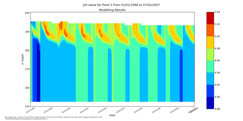
Depending on how long you model run the figure might look considerably different.
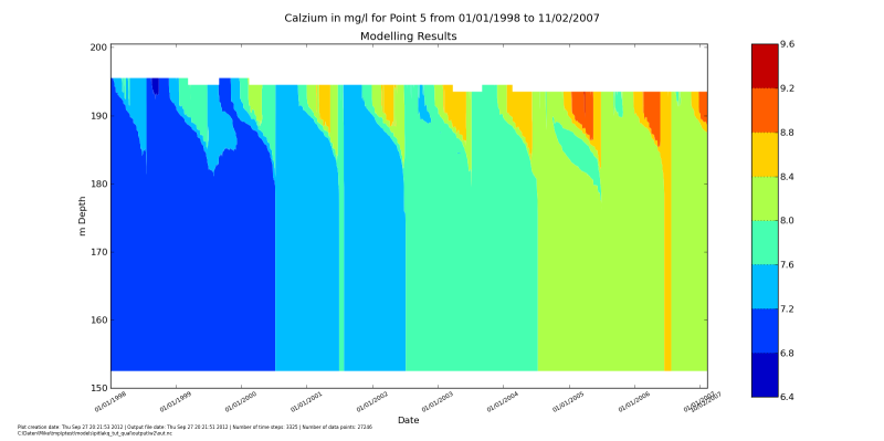
This script:
from pitlakq.postprocessing import depth_time_contour

species=[{"name": "ca", "levels": "auto"}]
depth_time_contour.main("../output/w2/out.nc", species=species, location=5)
after run pythont do_show_ca.py displays this figure
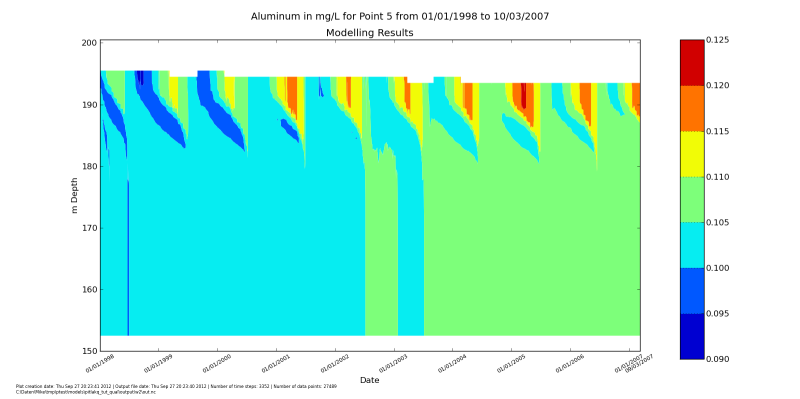
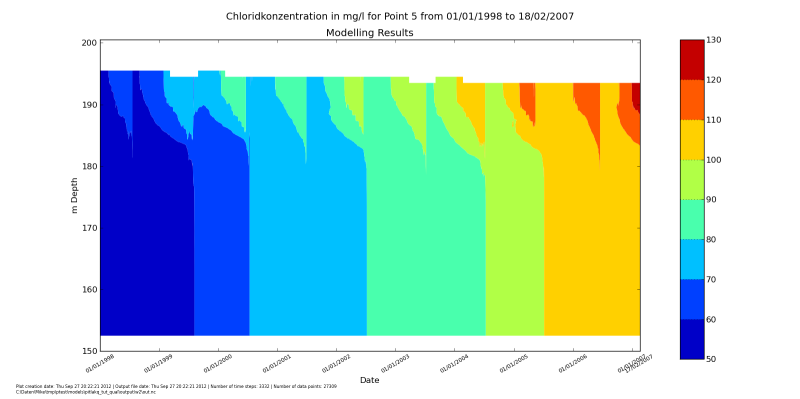
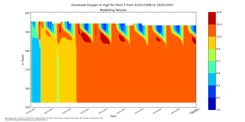
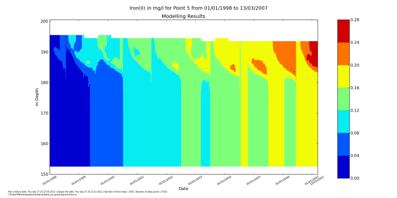
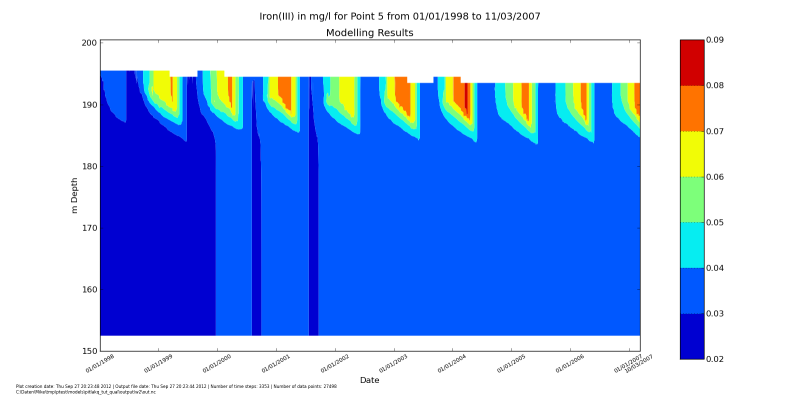
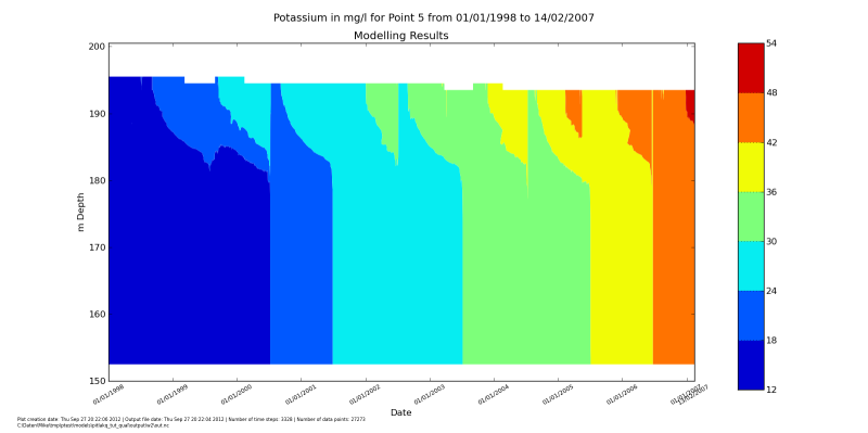
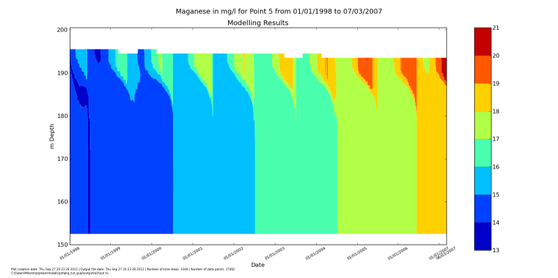
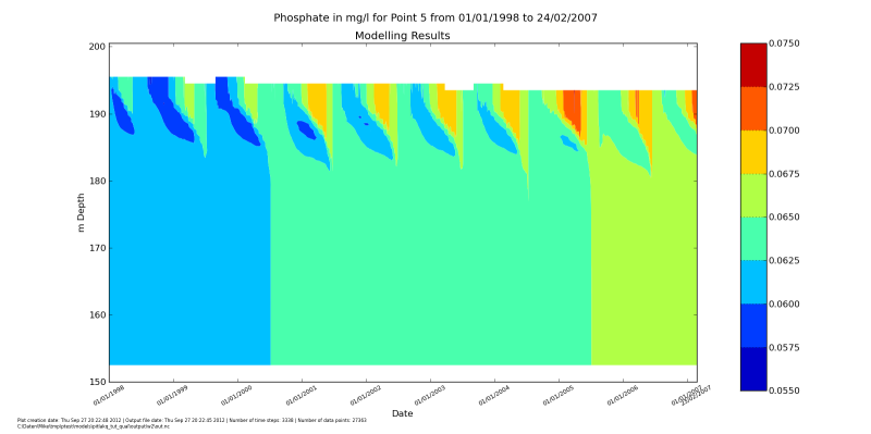
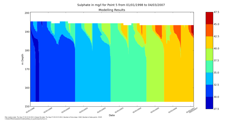
We can pout several constituents in one script:
from pitlakq.postprocessing import depth_time_contour

for name in ["na", "cl", "dox", "po4", "ca", "so4", "mg",
             "al", "fe3", "fe"]:
    species=[{"name": name, "levels": "auto"}]
    depth_time_contour.main("../output/w2/out.nc", species=species, location=5)
After running it with python do_show_many.py you should see the
windows popping up with these figures. After you close one, the next will up.
Making groundwater inflow a function of lake water level#
So far we have specified the groundwater inflow as a tributary inflow. For this we needed to provide the inflow for each desired time step. An alternative solution is to specify groundwater inflows as a function of lake water level.
First, we create a new project with pitlakq create pitlakq_tut_gwh.
We just copy the input folder from our former project
pitlakq_tut_qual. Introducing a new feature, it is always a good idea to
turn of water quality calculations for the first steps. This makes setting up
our new inflow simpler and test runs considerately faster.
To do this we just turn off the PHREEQC coupling. In pitlakq.yaml we set
this option for this to False:
couplings:
    phreeqc_coupling_lake:
        value: False
Furthermore, for know we also turn of kinetic calculations in W2 setting
the corresponding option in pitlakq.yaml to False:
lake:
    ...
    kinetics:
        value: False
Now we also turn off our groundwater inflow tributary. In w2.yaml we
set the number of tributaries to one.
bounds:
  ...
  number_of_tributaries:
      value: 1
And also change the tributary section to one tributary:
tributaries:
    number_of_tributaries:
        value: 1
    tributary_names:
        value:
            - mytribname
    tributary_segment:
        value:
            - 5
    tributary_inflow_placement:
        value:
            - 1 # density
    tributary_inflow_top_elevation:
        value:
            - 180
    tributary_inflow_bottom_elevation:
        value:
            - 155
Now we do a test run to see if the model still works:
pitlakq run pitlakq_tut_gwh
We turn on the option gwh in pitlakq.yaml:
gw:
    gwh:
        value: True
The only thing missing now is the actual input. We create a template input file with this script:
from pitlakq.preprocessing import create_xlsx_input

create_xlsx_input.main("pitlakq_tut_gwh")
Running it:
python do_gwh_xlsx.py
creates a file gwh_template.xlsx in input/gwh.
Rename this file to gwh.xlsx. This renaming is a safety measure to avoid
accidental re-creation of the file and loosing the entered in input.
This file has three tabs. The first one represents the zones:
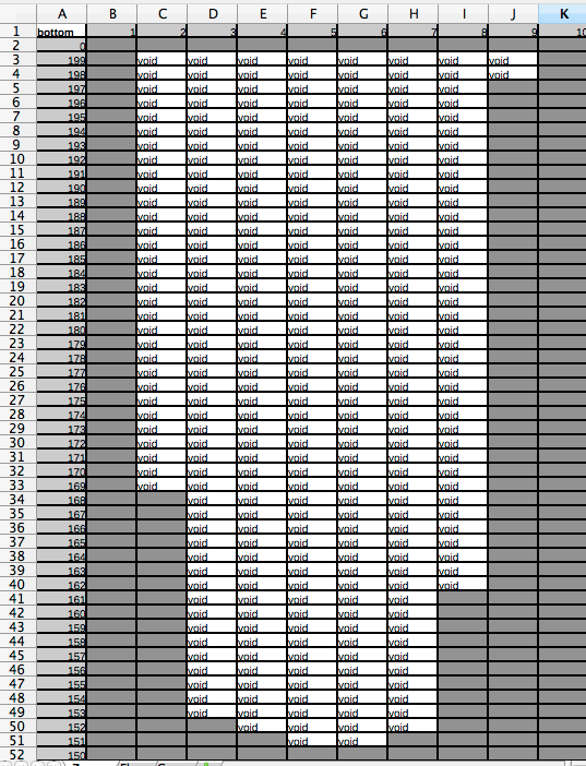
Only the white cells with the void inside are editable
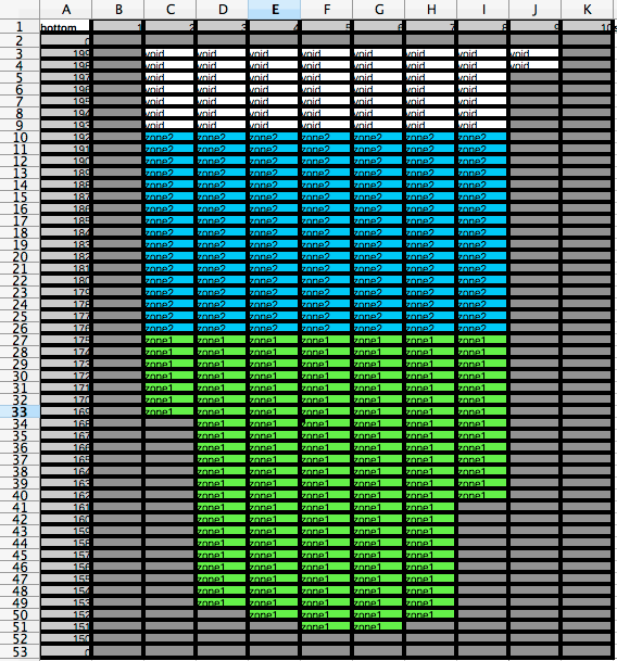
We added two zones. The color are optional and don’t mean anything to PITLAKQ. But the name is important. There is no limit on the number of zones as long as there are at least two cells in two adjacent layers in one zone. The inflows will be distributed over these cells according to there current water filled volume.
Inflows will activate only if the water level specified in the column
Level on the tab Flow will be reached by the lake water level. A soon
as the next level is reached, its inflow will be active and not the one below
anymore.
This way inflows can vary in many ways. Inflows can be negative which
results in groundwater outflow.
Zone name |
Level |
Flow |
|---|---|---|
zone1 |
155 |
0.02 |
zone1 |
160 |
0.01 |
zone1 |
170 |
0.05 |
zone1 |
180 |
0.001 |
zone2 |
180 |
0.002 |
zone2 |
185 |
0.001 |
zone2 |
190 |
-0.0 |
Each zone has one concentration specified in the tab Conc. We just use
the concentration from our groundwater tributary. This table shows the
first entries. Add all that from the original groundwater tributary file.
Zone name |
dissolved_oxygen |
ammonium |
nitrate_nitrite |
|---|---|---|---|
zone1 |
8 |
0 |
0.11 |
zone2 |
8 |
0 |
0.11 |
Now run the model. Modify levels and flow values to see the effect on the water level.
Finally, we can turn the water quality calculations back on.
Adding New Species to the Database#
PITLAKQ currently comes with 56 pre-defined solute species and 7 minerals. It is also possible to add user-defined species. There are several steps to incorporate own species in PITLAKQ. These species will be transported in CE-QUAL-W2 as tracers. All water quality processes will take place in PHREEQC. Furthermore, minerals that are allowed to form and precipitate can also be added. As with other minerals, they can be allowed to fully precipitate as soon as they are over-saturated or can be allowed to settle with potential dissolution on their way to the bottom if conditions change.
The next steps will modify files in the installation directory.
To avoid overwriting these files with defaults when updating pitlakq,
it is recommend to copy the directories <install_dir>/pitlakq/templates
and <install_dir>/pitlakq/resources into different locations.
These new locations need to be listed in your `.pitlakq file.
(See Initializing PITLAKQ for details.)
There are four steps involved in adding a new specie:
Add a new line in the file
resources/const_names.txtfor solute or in the fileresources/mineral_names.txtfor mineral species.Add a corresponding entry in the file
templates/w2.yaml.Add a corresponding entry in the file
templates/activeconst.txt.Optional: Update the PHREEQC database if it does not contain the new specie and the corresponding reactions yet.
These steps may get a bit more stream-lined in the future. Due to the fact that PITLAKQ was not designed from ground up for adding new species by the user, consolidating the information from steps 1. to 3. in one place would mean a major re-arrangement of the code base. Let’s go over the steps in detail.
Add a line to the files resources/const_names.txt or resources/mineral_names.txt#
The file resources/const_names.txt has this structure:
key    name          w2ssp  w2ssgw  phreeqc_name  molar_weight  rate_name

alkal  alkalinity    void   void    void          void          void
mn     manganese_II  mnssp  mnssgw  Mn(+2)        54.938        Mn_di
na     sodium        nassp  nassgw  Na            22.9898       void
There are more lines in this file. The three lines above are chosen to exemplify how different options look like.
The file resources/mineral_names.txt has this structure:
key     name            w2ssp     w2ssgw  phreeqc_name  molar_weight  rate_name

feoh3   iron_hydroxide  feoh3ssp  void    Fe(OH)3       106.871       Fe(OH)3(a)r
caco3   calcite         auto      void    Calcite       100.071       void
There are more lines in this file. The two lines above are chosen to exemplify how different options look like.
The columns have these meanings:
- key
Internal key used for CE-QUAL-W2 and other purposes. It must be unique. It is likely that one-letter names or very short names are already taken. PITLAKQ will warn you when this is the case. In this case, please choose another name. It is recommended to use a name that is as close as possible to the chemical symbol. Technically, any name consisting of English lowercase letters, digits and the underscore (
_) can be used. However, digits cannot appear at the beginning of a name.- name
A descriptive name for the specie. The name must be unique among the names in this column. The same name rules as for
keyapply.- w2ssp
Name used for exchange with PHREEQC. This is typically
<name>ssp. A specific name is only used for pre-defined species. As a user you can only choose between the optionautoorvoid. The entryautoshould be used for all species for which you want PHREEQC to use in its reactions. The actual name will be generated internally. Usingvoidin this column prevents the specie to be used for PHREEQC calculations. This is useful for species that don’t make sense in PHREEQC. For example,alkalinityin the example above is not used. It is the original alkalinity calculated in CE-QUAL-W2. It is contained only for technical reasons and serves no actual purpose for modeling. Due to the way the source code of CE-QUAL-W2 is structured, it would require a major re-write to turn off alkalinity with other means. Usingvoidcan be useful for other species such as tracers. This way you can add an unlimited number of tracers.- w2ssgw
Name used for exchange with groundwater. This is typically
<name>ssgw. A specific name is only used for pre-defined species. As a user you can only choose between the optionautoorvoid. The entryautoshould be used for all species for which the groundwater should act as source and sink. The actual name will be generated internally. Usingvoidin this column prevents any exchange with the groundwater for this specie. This is useful for minerals that can be transported in the lake but typically not in the groundwater due to velocities that are orders of magnitude smaller.- phreeqc_name
This is the name of the specie used in PHREEQC. It must appear in the database in
SOLUTION_MASTER_SPECIESfor solutes or inPHASESfor minerals. See the PHREEQC manual for more details.- molar_weight
The molar weight of the specie. This must be the same value as used in the PHREEQC database. So far there are no know use cases where this value differs from the one in PHREEQC. It you know of one, please tell the model developers.
- rate_name
This is an alternative name for the specie used in PHREEQC’s rate reactions. You must name the specie matching the corresponding entry under
KINETICSin the PHREEQC database.
A typical entry in resources/const_names.txt would look like this:
key name      w2ssp   w2ssgw  phreeqc_name    molar_weight    rate_name

.... other lines here ....

van vanadium  auto    auto    V               50.9415         void
Since v is already used in CE-QUAL-W2 (PITLAKQ will warn you about it),
we choose van for key. The entry for name is just the lower case
version of the chemical name. The entry for w2ssp must be auto because
we want our species to react in PHREEQC. Likewise, the entry for w2ssgw is
also auto because we would like the exchange with groundwater to be possible.
It can be enabled and disabled for each model but must be auto, otherwise
it cannot be enabled at all. The PHREEQC name is just the normal chemical name
and you must use the same name as in the PHREEQC database.
The molar weight is copied from the PHREEQC database. We don’t want to use
kinetic rate reactions, therefore rate_name is void.
Adding a new line at the end of the file resources/mineral_names.txt should
look like this:
key     name            w2ssp     w2ssgw  phreeqc_name  molar_weight  rate_name

.... other lines here ....

caco3   calcite         auto      void    Calcite       100.071       void
The meanings are the same as above. We choose a unique name for the key.
In our case the lowercase version of the chemical formula. The name is the
lowercased PHREEQC name. We want reactions in PHREEQC, hence auto for
w2ssp. Minerals typically are not transported in the groundwater, therefore
void in w2ssgw. The molar weight is again the value PHREEQC uses.
We also do not want rate reactions and set rate_name to void.
Add an entry in templates/w2.yaml#
We need to tell CE-QUAL-W2 about the new specie. We need to add an entry
inside the group initial_concentrations. Going with our example
for vanadium it would look like this:
initial_concentrations:
    # many more entries here
    vanadium:
        default: 0.0
        w2_code_name: van
        dimension:
            - number_of_layers
            - number_of_segments
Unless you want a default initial concentration different from zero, add
default: 0.0. The entry for w2_code_name must be the same as in the
column key in resources/const_names.txt or
resources/mineral_names.txt. Always use the same entries for dimension.
Add an entry in templates/activeconst.txt#
The file templates/activeconst.txt looks like this:
constituent_name active_constituents initial_concentration inflow_active_constituents tributary_active_constituents precipitation_active_constituents
.... other lines here ....
iron_II          0                   0                     0                          0                             0
.... other lines here ....
silver           0                   0                     0                          0                             0
.... other lines here ....
Per default all species should be inactive. Using this file copied to your model input, you can activate any specie you need for any if the columns.
Adding a new specie is simple. Just use the name you entered in the column
name in resources/const_names.txt or resources/mineral_names.txt
and copy all the zeros from the line above:
constituent_name active_constituents initial_concentration inflow_active_constituents tributary_active_constituents precipitation_active_constituents
.... other lines here ....
vanadium           0                   0                     0                          0                             0
Update the PHREEQC database#
You may need to update your PHREEQC database to reflect your changes. You don’t need to do anything, if the database already contains all species you added including all the reactions that are needed for your site.
You can also specify a different database. Just add this to your
pitlakq.yaml:
phreeqc:
    # more lines here
    phreeqc_database_name:
        value: my_database.dat ## default is phreeqc_w2.dat
You need to copy the database file my_database.dat into the directory
resources of you PITLAKQ install. Refer to .pitlakq where this is
on your computer.
Pit Wall Loading#
Needed information#
The water quality of a pit lake can be significantly influenced by material from the pit wall entering the lake. PITLAKQ offers a way to simulate these loadings. There are several prerequisites that need to be satisfied for the modeling approach to work:
You need to specify loading rates expressed in mass per area per time from the pit walls for all species that you would like to model. Such loading rates are typically measured in laboratory experiments. The rates need to be assigned to pit wall zones. There is no limit on the number of zones. There can be as few as one zone, covering all pit walls, or as many as dozens, hundreds, or thousands of zones if such detailed information is available.
You need to specify surface areas of the pit wall for each zone for different lake water levels. There is no limit on the number of lake water levels with different surface areas you can specify. However, there must be at least two levels. This surface areas will be used to calculate the effective loadings for each zone for the current water level.
You also need to specify planar areas in the fashion as surface areas. These planar areas will be used to calculate the run off from the pit walls using the precipitation specified in the model input for the CE-QUAL-W2 part of PITLAKQ.
The procedure#
PITLAKQ is calculating the following:
For each loading time step, typically one day but it can be set by the user, the model determines the surface area of each zone. Each area is multiplied by the given loading rate for this zone and the elapsed time (one day for our example case). These masses are accumulated to be added to the lake as soon as there is runoff.
The precipitation for the time period is calculated. If there is no precipitation, nothing happens. If there is precipitation, it will be multiplied with the planar area of each zone to yield the water volume supplied by each zone.
The water volume is added to a specified region of the lake. This region is determined by a user-defined number of layers counted from the lake surface and active lake segments per zone. In addition, the lake receives the accumulated masses from step 1. and an amount of heat provided by a given temperature multiplied by the volumes. After adding the masses to the lake, the accumulated masses are set to zero. This means the accumulation can begin anew with the next time step.
For example, if there is a 10-day period without precipitation, the model would accumulate masses for all species for all zones according to the specified loading rates and current surface areas for all zones. After 10 days the calculated precipitation volumes for each zone would carry these masses into the lake. For wet climates with frequent precipitation this results in a steady loading from the pit walls. On the other hand, for dry climates with infrequent precipitation this simulates longer periods without any loading followed by short peaks of loading.
Model input#
The input for the loading is contained in the file loading.xlsx in the
directory input/loading. The tab “Area” holds a table of surface areas
and planar areas in m2 for each desired water table as well as start
and end segment of the lake in between which the load should be applied.
For one zone this table could look like this:
water_level |
zone1_planar |
zone1_surface |
zone1_start_segment |
zone1_end_segment |
|---|---|---|---|---|
152 |
0 |
0 |
4 |
5 |
155 |
73278.2 |
97704.3 |
4 |
5 |
153 |
69492.0 |
92656.0 |
6 |
8 |
154 |
67777.0 |
90370.4 |
6 |
8 |
155 |
67048.0 |
89398.1 |
6 |
8 |
Typically there are more lines in a table, covering the whole expected range of water table changes. Using a value of zero for areas effectively turns them off for this water table. This allows to represent inactive areas for certain areas. A table for three zones would have this header:
Header |
|
|---|---|
water_level |
|
zone1_planar |
|
zone2_planar |
|
zone3_planar |
|
zone1_surface |
|
zone2_surface |
|
zone3_surface |
|
zone1_start_segment |
|
zone1_end_segment |
|
zone2_start_segment |
|
zone2_end_segment |
|
zone3_start_segment |
|
zone3_end_segment |
The numbers for the areas need to be supplied by the user. Currently, there is no extra tool for preprocessing that would generate the area information from bathymetry information. Using GIS software, generation of the area information should be straight forward.
The table under the tab “Conc” holds the loading data in g/m2/s.
Each zone name that was used in the table under tab “Area” must appear in the
column zone. All species that are to be active for loading have to given in
the columns of the table as headings:
zone |
cobalt |
silver |
zinc |
tracer |
calcium |
|---|---|---|---|---|---|
zone1 |
1.00E-011 |
1.00E-010 |
1.00E-010 |
1.00E-010 |
1.00E-010 |
zone2 |
5.00E-011 |
1.00E-010 |
4.00E-010 |
1.00E-010 |
1.00E-010 |
zone3 |
0 |
1.00E-010 |
1.00E-011 |
1.00E-010 |
1.00E-010 |
In addition, all species in this table must be turned on using a 1 for
active_constituents in the file input/w2/activeconst.txt in your
model input. Please do not turn them on as default in
resources\activeconst.txt as this would affect all other models, which is
typically undesirable.